Analyzing 10x Genomics scRNA-seq Data#
[1]:
import precellar
Download the seqspec file corresponding to the 10x Genomics v3 chemistry.
[2]:
assay = precellar.Assay('https://raw.githubusercontent.com/regulatory-genomics/precellar/refs/heads/main/seqspec_templates/10x_rna_v3.yaml')
Download the FASTQ files from the 10k PBMC dataset: https://cf.10xgenomics.com/samples/cell-exp/6.1.0/500_PBMC_3p_LT_Chromium_X/500_PBMC_3p_LT_Chromium_X_fastqs.tar.
[3]:
fq1 = [
    '/data2/data/Public_data/10X_genomics_gex/fastq/500_PBMC_3p_LT_Chromium_X/500_PBMC_3p_LT_Chromium_X_S4_L003_R1_001.fastq.gz',
    '/data2/data/Public_data/10X_genomics_gex/fastq/500_PBMC_3p_LT_Chromium_X/500_PBMC_3p_LT_Chromium_X_S4_L004_R1_001.fastq.gz',
]
fq2 = [
    '/data2/data/Public_data/10X_genomics_gex/fastq/500_PBMC_3p_LT_Chromium_X/500_PBMC_3p_LT_Chromium_X_S4_L003_R2_001.fastq.gz',
    '/data2/data/Public_data/10X_genomics_gex/fastq/500_PBMC_3p_LT_Chromium_X/500_PBMC_3p_LT_Chromium_X_S4_L004_R2_001.fastq.gz',
]
Update the Assay object to include the path to the fastq files.
[4]:
assay.add_illumina_reads('rna')
assay.update_read('rna-R1', fastq=fq1)
assay.update_read('rna-R2', fastq=fq2)
assay
[2025-10-07T11:56:33Z INFO] The read length of rna-R1 was inferred to be 28.
[2025-10-07T11:56:35Z INFO] The read length of rna-R2 was inferred to be 90.
[4]:
10xRNAv3
└── rna(153-1150)
    ├── rna-illumina_p5(29)
    ├── rna-truseq_read1(29) [↓rna-R1(28)✓]
    ├── rna-cell_barcode(16)
    ├── rna-umi(12)
    ├── rna-polyT(10-250)
    ├── rna-cDNA(1-1000)
    ├── rna-truseq_read2(34) [↑rna-R2(90)✓, ↓rna-I1(8)✗]
    ├── rna-index7(8)
    └── rna-illumina_p7(24)
Perform read alignment, filtering, and gene quantification for 10x Genomics single-cell RNA-seq data using precellar. The results will be saved in an AnnData file.
Note the progress bar does not display correctly in jupyter notebooks. It is better to run this script in a terminal.
[5]:
qc = precellar.align(
    assay,
    precellar.aligners.STAR("/data/Public/STAR_reference/refdata-gex-GRCh38-2024-A/star"),
    output="gene_matrix.h5ad",
    output_type="gene_quantification",
    num_threads=32,
)
[2025-10-07T11:56:38Z INFO] Using default modality: rna
[2025-10-07T11:56:41Z INFO] Counting barcodes in read rna-R1...
[2025-10-07T11:57:21Z INFO] 93.80% of sequences have an exact match in whitelist 'rna-cell_barcode'. Number of unique barcodes: 25253.
[2025-10-07T11:57:22Z INFO] Aligning 75,670,679 reads to reference genome ...
[2025-10-07T11:57:36Z INFO] Found 86.127% sense and 13.873% antisense alignments
[2025-10-07T11:57:36Z INFO] Chemistry strandness is set to: Forward
Print the QC metrics.
[7]:
qc
[7]:
{'alignment': {'frac_confidently_mapped': 0.790326533486316,
  'frac_mitochondrial': 0.08258507615204208,
  'frac_properly_paired': 0.0,
  'frac_unmapped': 0.09483609480246813,
  'frac_valid_barcode': 0.9655930931979612,
  'mapped_reads': 67947954,
  'sequenced_read_pairs': 0,
  'sequenced_reads': 75670679},
 'fastq': {'frac_q30_bases': {'barcode': 0.9565258807179462,
   'read2': 0.8897475697878229,
   'umi': 0.9537967803883457}},
 'gene_quantification': {'frac_transcriptomic': 0.6503691476060364,
  'mapping': {'frac_antisense': 0.09794439666650805,
   'frac_discordant': 0.0074563887552799675,
   'frac_exonic': 0.30161883442330417,
   'frac_intergenic': 0.04225893096585006,
   'frac_intronic': 0.178415684627331,
   'frac_mixed': 0.15963624431069265,
   'frac_multimapped': 0.07599115107715632,
   'frac_spanning': 0.010698384244708575},
  'quantification': {'frac_duplicates': 0.7752581157244781,
   'frac_spliced': 0.3584300920245426,
   'frac_unspliced': 0.3483781220223212}}}
We will now use SnapATAC2 to perform downstream analysis on the generated h5ad file. SnapATAC2 can be downloaded here: scverse/SnapATAC2.
[8]:
import snapatac2 as snap
import numpy as np
import hdf5plugin
[9]:
adata = snap.read('gene_matrix.h5ad', backed=None)
adata
[9]:
AnnData object with n_obs × n_vars = 31989 × 38606
    var: 'gene_name'
    uns: 'reference_sequences'
    obsm: 'fragment_single'
    layers: 'spliced', 'unspliced'
[10]:
gene_count = np.ravel(adata.X.sum(axis=1))
adata = adata[gene_count > 1000, :].copy()
adata
[10]:
AnnData object with n_obs × n_vars = 589 × 38606
    var: 'gene_name'
    uns: 'reference_sequences'
    obsm: 'fragment_single'
    layers: 'spliced', 'unspliced'
[11]:
adata.X = np.log1p(adata.X)
[12]:
snap.tl.spectral(adata, features=None)
snap.pp.knn(adata)
snap.tl.umap(adata)
snap.tl.leiden(adata)
/data/kzhang/micromamba/lib/python3.10/site-packages/sklearn/utils/deprecation.py:132: FutureWarning: 'force_all_finite' was renamed to 'ensure_all_finite' in 1.6 and will be removed in 1.8.
  warnings.warn(
/data/kzhang/micromamba/lib/python3.10/site-packages/umap/umap_.py:1945: UserWarning: n_jobs value 1 overridden to 1 by setting random_state. Use no seed for parallelism.
  warn(f"n_jobs value {self.n_jobs} overridden to 1 by setting random_state. Use no seed for parallelism.")
Visualize the cell clusters using UMAP.
[13]:
snap.pl.umap(adata, color='leiden')
Precellar not only computes gene expression counts but also retains the raw read coverage for each cell. To demonstrate this feature, we will plot the raw signal coverage of a specific gene across different cell clusters.
For example, we will use the gene CD19, which is a marker for B cells.
[14]:
snap.pl.coverage(adata, region='chr16:28931971-28939342', groupby='leiden')
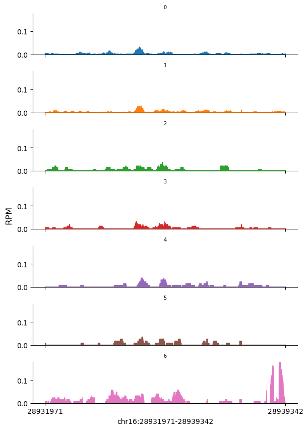
As shown in the plot above, the cluster 6 is likely to be B cells, as they show high coverage over the gene body of CD19.